2. ESDC Description
2.1. Macro Structure
The data is organised in the described 4-dimensional form x(u,v,t,k), but additionally each data stream k is assigned to one of the subsystems of interest:
- Land surface
- Atmospheric forcing
- Socio-economic data
2.2. Spatial and Temporal Coverage
The fine grid of the ESDC has a spatial resolution of 0.083° (5”), which is properly nested within a coarse grid of 0.25° (15”). Hence, the ESDC is available in two versions
- High resolution version: 0.083° (5”) spatial resolution,
- Low resolution version: 0.25° (15”) spatial resolution.
While the latter contains all variables, the former only comprises those variables that are natively available at this resolution. The high-resolution data are nested on the low-resolution data set such that one can analyse these in tandem. In particular data from the socio-economic subsystem are often organised according to administrative units, typically national states, rather than on regular grids. These data are dispersed to the coarse grid by means of a national state mask, which is created by assigning a national state property to each grid point.
The temporal resolution is 8 days.
The time span currently covered is 2001-2011. We are dedicated to expand this period on both ends, but to preserve the ESDC’s characteristics, a reasonable coverage of data streams is required.
2.3. Format and Structure
The binary data format for the Earth System Data Cube (ESDC) in the CAB-LAB project is netCDF 4 classic, where the term classic stands for an underlying HDF-5 format accessed by a netCDF 4 API.
The netCDF file’s content and structure follows the CF-conventions. That is, there are are always at least three dimensions defined
lon- Always the inner and therefore fastest varying dimension. Defines the raster width of spatial images.lat- Always the second dimension. Defines the raster height of spatial images.time- Time dimension.
There are 1D-variables related to each dimension providing its actual values:
lon(lon)andlat(lon)- longitudes and latitudes in decimal degrees defined in a WGS-84 geographical- coordinate reference system. The spatial grid is homogeneous with the distance between two grid points referred to as the ESDC’s spatial resolution.
start_time(time)andend_time(time)- Period start and end times of a datum given in- days since 2001-01-01 00:00. The increments between two values in time are identical and referred to as the ESDC’s temporal resolution.
There is usually only a single geophysical variable with shape(time, lat, lon) represented by each
netCDF file. So each netCDF file is composed of length(time) spatial images of that variable, where each image
of size length(lon) x length(lat) pixels has been generated by aggregating all source data contributing
to the period given by the ESDC’s temporal resolution.
To limit the size of individual files, the geophysical variables are stored in one file per year. For example, if the temporal resolution is 0.25 degrees and the the spatial resolution is an 8-day period then there will be up to 46 images of 1440 x 720 pixels in each annual netCDF file. These annual files are stored in dedicated sub-directories as follows:
<cube-root-dir>/
    cube.config
    data/
        LAI/
            2001_LAI.nc
            2002_LAI.nc
            ...
            2011_LAI.nc
        Ozone/
            2001_Ozone.nc
            2002_Ozone.nc
            ...
            2011_Ozone.nc
        ...
The names of the geophysical variable in a netCDF file must match the name of the corresponding sub-directory and the file name.
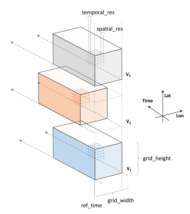
The text file cube.config contains a Data Cube’s static configuration such as its temporal and spatial resolution.
Also the spatial coverage is constant, that is, all spatial images are of the same size. Where actual data is missing,
fill values are inserted to expand a data set to the dimensions of the Data Cube.
The fill values in the Data Cube are identical to the ones used in the Data Cube’s sources. The same holds for the data types.
While all images for all time periods have the same size, the temporal coverage for a given variable may vary.
Missing spatial images for a given time period are treated as images with all pixels set to a fill value.
The following table contains all possible configuration parameters:
| Parameter | Default Value | Description |
|---|---|---|
temporal_res |
8 |
The constant temporal resolution given as integer days. |
calendar |
'gregorian' |
Defines the Data Cube’s time units. |
ref_time |
datetime(2001, 1, 1) |
The Data Cube’s time unit is days since a reference date/time. |
start_time |
datetime(2001, 1, 1) |
The start date/time of contributing source data. |
end_time |
datetime(2011, 1, 1) |
The end date/time of contributing source data. |
spatial_res |
0.25 |
The constant spatial resolution given in decimal degrees. |
grid_x0 |
0 |
The spatial grid’s X-offset. |
grid_y0 |
0 |
The spatial grid’s Y-offset. |
grid_width |
1440 |
The spatial grid’s width. Must always be 360 / spatial_res. |
grid_height |
720 |
The spatial grid’s height. Must always be 180 / spatial_res. |
variables |
None |
The variables contained in the Data Cube. |
file_format |
'NETCDF4_CLASSIC' |
The target binary file format. |
compression |
False |
Whether or not the target binary files should be compressed. |
model_version |
'0.1' |
The version of the Data Cube model and configuration. |
2.4. Processing Applied
The Data Cube is generated by the cube-cli tool. This tools creates a Data Cube for a given configuration
and can be used to subsequently add variables, one by one, to the Data Cube. Each variable is read from its specific data source and
transformed in time and space to comply to the specification defined by the target Data Cube’s configuration.
The general approach is as follows: For each variable and a given Data Cube time period: * Read the variable’s data from all contributing sources that have an overlap with the target period; * Perform temporal aggregation of all contributing spatial images in the original spatial resolution; * Perform spatial upsampling or downsampling of the image aggregated in time; * Mask the resulting upsampled/downsampled image by the common land-sea mask; * Insert the final image for the variable and target time period into the Data Cube.
The following sections describe each method used in more detail.
2.4.1. Gap-Filling Approach
The current version (version 0.1, Feb 2016) of the ESDC does not explicitly fill gaps. However, some gap-filling occurs during temporal aggregation as described below. The CAB-LAB team may provide gap-filled ESDC versions at a later point in time of the project. Gap-filling is part of the Data Analytics Toolkit and is thus not tackled during Data Cube generation to retain the information on the original data coverage as much as possible.
For future Data Cube versions per-variable gap-filling strategies may be applied. Also, only a spatio-temporal region of interest may be gap-filled while cells outside this region may be filled by global default values. An instructive example of such an approach would be the gap-filling of a leaf area index (LAI) data set, which only takes place in mid-latitudes while gaps in high-latitudess are filled with zeros.
2.4.2. Temporal Resampling
Temporal resampling starts on the 1st January of every year so that all the i-th spatial images in the ESDC refer to the same time of the year, namely starting i x temporal resolution. Source data is collected for every resulting ESDC target period. If there is more than one contribution in time, then each contribution is weighted according to the temporal overlap with the target period. Finally, target pixel values are computed by averaging all weighted values in time not masked by a fill value. By doing so, some temporal gaps are filled implicitly.
2.4.3. Spatial Resampling
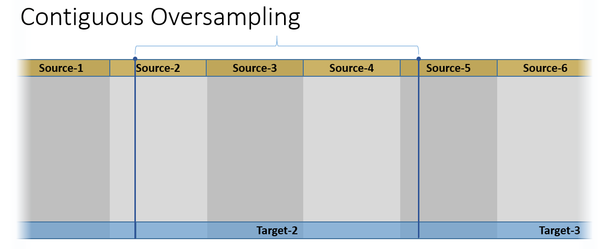
Spatial resampling occurs after temporal resampling only if the ESDC’s spatial resolution differs from the data source resolution.
If the ESDC’s spatial resolution is higher than the data source’s spatial resolution, source images are upsampled by rescaling hereby duplicating original values, but not performing any spatial interpolation.
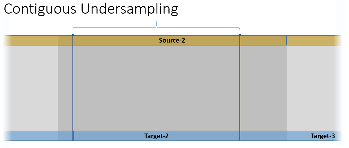
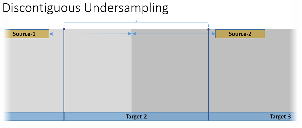
If the ESDC’s spatial resolution is lower than the data source’s spatial resolution, source images are downsampled by aggregation hereby performing a weighted spatial averaging taking into account missing values. If there is not an integer factor between the source and the Data Cube resolution, weights will be found according to the spatial overlap of source and target cells.
 |
 |
 |
 |
2.4.4. Land-Water Masking
After spatial resampling, a land-water mask is applied to individual variables depending on whether a variable is defined for water surfaces only, land surfaces only, or both. A common land-water mask is used for all variables for a given spatial resolution. Masked values are indicated by fill values.
2.4.5. Constraints and Limitations
The ESDC approach of transforming all variables onto a common grid greatly facilitates handling and joint analysis of data sets that originally had different characteristics and were generated under different assumptions. Regridding, gap-filling, and averaging, however, may alter the information contained in the original data considerably.
The main idea of the ESDC is to provide a consistent and synoptic characterisation of the Earth System at given time steps to promote global analyses. Therefore, conducting small-scale, high frequency studies that are potentially highly sensible to individual artifacts introduced by data transformation is not encouraged. The cautious expert user may hence carefully check phenomena close to the Land-Sea mask or in data sparse regions of the original data. If in doubt, suspicious patterns in the ESDC or unexpected analytical results should be verified with the source data in the native resolution. We try here as much as possible to conserve the characteristics of the original data, while facilitating data handling and analysis by transformation.
This is a difficult balance to strike that at times involves inconvenient trade-offs. We thus embrace transparency and reproducibility to enable the informed user to evaluate the validity and consistency of the processed data and strive to offer options for data transformation wherever possible.
2.5. Cube Data Variables
| Project | Name in ESDC | Description | URL | References |
|---|---|---|---|---|
| GLEAM | evaporative_stress | Evaporative Stress Factor | http://www.gleam.eu | Martens, B., Miralles, D.G., Lievens, H., van der Schalie, R., de Jeu, R.A.M., Fernández-Prieto, D., Beck, H.E., Dorigo, W.A., and Verhoest, N.E.C.: GLEAM v3: satellite-based land evaporation and root-zone soil moisture, Geoscientific Model Development, 10, 1903–1925, 2017. |
| evaporation | Evaporation | |||
| snow_sublimation | Snow Sublimation | |||
| potential_evaporation | Potential Evaporation | |||
| interception_loss | Interception Loss | |||
| bare_soil_evaporation | Bare Soil Evaporation | |||
| open_water_evaporation | Open-water Evaporation | |||
| surface_moisture | Surface Soil Moisture | |||
| transpiration | Transpiration | |||
| root_moisture | Root-Zone Soil Moisture | |||
| GFED4 | burnt_area | Burnt Area based on the GFED4 fire product. | http://www.globalfiredata.org/ | Giglio, Louis, James T. Randerson, and Guido R. Werf. “Analysis of daily, monthly, and annual burned area using the fourth‐generation global fire emissions database (GFED4).” Journal of Geophysical Research: Biogeosciences 118.1 (2013): 317-328. |
| c_emissions | Carbon emissions by fires based on the GFED4 fire product. | |||
| ESA Aerosol CCI | aerosol_optical_thickness_865 | Aerosol optical thickness derived from the dataset produced by the Aerosol CCI project. | http://www.esa-aerosol-cci.org/ | Holzer-Popp, T., de Leeuw, G., Griesfeller, J., Martynenko, D., Klueser, L., Bevan, S., et al. (2013). Aerosol retrieval experiments in the ESA Aerosol_cci project. Atmospheric Measurement Techniques, 6, 1919-1957. doi:10.5194/amt-6-1919-2013. |
| aerosol_optical_thickness_1610 | Aerosol optical thickness derived from the dataset produced by the Aerosol CCI project. | |||
| aerosol_optical_thickness_550 | Aerosol optical thickness derived from the dataset produced by the Aerosol CCI project. | |||
| aerosol_optical_thickness_659 | Aerosol optical thickness derived from the dataset produced by the Aerosol CCI project. | |||
| aerosol_optical_thickness_555 | Aerosol optical thickness derived from the dataset produced by the Aerosol CCI project. | |||
| GlobTemperature | land_surface_temperature | Advanced Along Track Scanning Radiometer pixel land surface temperature product | http://data.globtemperature.info/ | Jiménez, C., et al. “Inversion of AMSR‐E observations for land surface temperature estimation: 1. Methodology and evaluation with station temperature.” Journal of Geophysical Research: Atmospheres 122.6 (2017): 3330-3347. |
| ERAInterim | air_temperature_2m | Air temperature at 2m from the ERAInterim reanalysis product. | http://www.ecmwf.int/en/research/climate-reanalysis/era-interim | Dee, D.P. et al. 2011 http://onlinelibrary.wiley.com/doi/10.1002/qj.828/abstract |
| SoilMoisture CCI | soil_moisture | Soil moisture based on the SOilmoisture CCI project | http://www.esa-soilmoisture-cci.org | Liu, Y.Y., Parinussa, R.M., Dorigo, W.A., De Jeu, R.A.M., Wagner, W., McCabe, M.F., Evans, J.P., and van Dijk, A.I.J.M. (2012): Trend-preserving blending of passive and active microwave soil moisture retrievals; Liu, Y.Y., Parinussa, R.M., Dorigo, W.A., De Jeu, R.A.M., Wagner, W., van Dijk, A.I.J.M., McCabe, M.F., & Evans, J.P. (2011): Developing an improved soil moisture dataset by blending passive and active microwave satellite based retrievals. Hydrology and Earth System Sciences, 15, 425-436. |
| GlobVapour | water_vapour | Total column water vapour based on the GlobVapour CCI product. | http://www.globvapour.info/ | Schneider, Nadine, et al. “ESA DUE GlobVapour water vapor products: Validation.” AIP Conference Proceedings. Vol. 1531. No. 1. 2013. |
| Ozone CCI | ozone | Atmospheric ozone based on the Ozone CCI data. | http://www.esa-ozone-cci.org/ | Laeng, A., et al. “The ozone climate change initiative: Comparison of four Level-2 processors for the Michelson Interferometer for Passive Atmospheric Sounding (MIPAS).” Remote Sensing of Environment 162 (2015): 316-343. |
| GlobAlbedo | white_sky_albedo | White sky albedo derived from the GlobAlbedo CCI project dataset | http://www.globalbedo.org/ | Muller, Jan-Peter, et al. “The ESA GLOBALBEDO project for mapping the Earth’s land surface albedo for 15 years from European sensors.” Geophysical Research Abstracts. Vol. 13. 2012. |
| black_sky_albedo | Black sky albedo derived from the GlobAlbedo CCI project dataset | |||
| FLUXCOM | net_ecosystem_exchange | Net carbon exchange between the ecosystem and the atmopshere. | http://www.fluxcom.org/ | Tramontana, Gianluca, et al. “Predicting carbon dioxide and energy fluxes across global FLUXNET sites with regression algorithms.” (2016). |
| terrestrial_ecosystem_respiration | Total carbon release of the ecosystem through respiration. | |||
| gross_primary_productivity | Gross Carbon uptake of of the ecosystem through photosynthesis | |||
| latent_energy | Latent heat flux from the surface. | |||
| sensible_heat | Sensible heat flux from the surface | |||
| GPCP | precipitation | Precipitation based on the GPCP dataset. | http://precip.gsfc.nasa.gov/ | Adler, Robert F., et al. “The version-2 global precipitation climatology project (GPCP) monthly precipitation analysis (1979-present).” Journal of hydrometeorology 4.6 (2003): 1147-1167. |
| GlobSnow | fractional_snow_cover | Grid cell fractional snow cover based on the Globsnow CCI product. | http://www.globsnow.info/ | Luojus, Kari, et al. “ESA DUE Globsnow-Global Snow Database for Climate Research.” ESA Special Publication. Vol. 686. 2010. |
| snow_water_equivalent | Grid cell fractional snow cover based on the Globsnow CCI product. |